History of package tzf

The core development of tzf and related projects has stabilized. The previous article contains sporadic information about the development and design process:

• 2022-05-29,在 Go 中将经纬度转时区
• 2022-08-01,Python 中经纬度转时区新的选择
• 2022-08-27,用 Go 编写 Python 扩展
• 2022-09-10,tzf 预览图制作
• 2022-11-24,tzfpy Rust 重写

This article is the final summary, from the start-up of the project to the gradual optimization and evolution.

We used to use  timezonefinder to convert longitude&latitude to timezone names. And it could be very slow around polygon borders. In previous versions, the query of the edge of the polygon may need to be 200ms or even 800ms. Inversion @6.1.0 it switched to the Ray Cast algorithm implemented by C, but it was still not so stable. The time-consuming gap between the fastest and slowest was relatively large, so I set out to develop my own library for converting longitude and latitude to time zones.

I have experience converting GPS coordinates to Chinese administrative divisions (a Chinese introduction can be found here), which includes the problem of Point in polygon andRay casting algorithm. So in theory, all I need is the timezone’s shapes data. We need great thanks for@evansiroky who maintains a repository namedtimezone-boundary-builder that keep tracking Timezone Database’s release while maintaining GeoJSON and ShapeFile data files release for years, and data files are licensed under theOpen Data Commons Open Database License (ODbL), so we can use these files legally.

I choose to process GeoJSON file because I’m more familiar with it. This file is about 45MB after compression and 155MB after decompression, which is too large for the project, so the first problem is how to reduce the data volume.

One of the simplest ideas is to store it in a more efficient binary encoding format. My team was familiar with Protocol Buffers, so I wrote thetzinfo.proto file. It should be noted that in GeoJSON’s definition ofRFC 7946, a Polygon is made up of multiple linear rings: the first represents the outer boundary of the polygon, and the rest represent internal holes inside the polygon. This kind of data is repeated repeated Point with Protocol Buffers syntax, which is not supported by Protocol Buffers. It needs to be split into two fields to represent:

message Point {
  float lng = 1;
  float lat = 2;
}

message Polygon {
  repeated Point points = 1;
  repeated Polygon holes = 2;
}

message Timezone {
  repeated Polygon polygons = 1;
  string name = 2;
}

message Timezones {
  repeated Timezone timezones = 1;
}

After processing, the file volume has been reduced by about 80MB. It takes about 900MB for this part of the data to be fully loaded into memory. The volume is too large and needs to be reduced. If you look closely at the coordinates in the GeoJSON file, you will find that their point spacing is relatively dense, but such high precision is unnecessary in production use cases. Therefore, the first optimization strategy is to reduce the amount of data at the point.

So how to effectively reduce the number of polygon scattering points? The most commonly used algorithm in this field is theRamer–Douglas–Peucker algorithm:

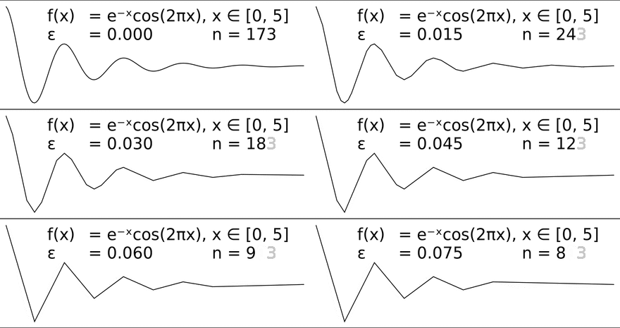
As the GIF demonstrates, a complex curve can be simplified to fewer points while maintaining a rough shape. After the filtering of the algorithm, the volume of the file has been reduced to 11MB.

At this point, I wondered whether the 11MB binary file was still a little large in various binary distribution scenarios, so I investigated the coordinate data compression methods and found thatPolyline is more suitable. This is Google Maps’ algorithm for compressing continuous coordinates. The principle is that all points except for the first point are stored as offset relative to the previous point, and then the offset is extracted through bit operation to calculate the binary sequence and processed into ASCII. After a single data processing, the time zone polygon data file is compressed to 4.6MB, which is very friendly for binary distribution.

In fact, a usable time zone library had emerged, and the query performance was slightly faster than that of timezonefinder. However, as mentioned earlier, production use cases involve high-concurrency traffic pressure. The execution frequency of this part is very high, and the faster the better. Because the Ray casting algorithm has $O(n^2)$ time complexity, so it is best to minimize how often this part executes, which led to designing an index mechanism for time zones.

According to the experience of administrative divisions, RTree should be enabled here to avoid traversing all polygons. But the improvement was not significant in benchmarks on global city data. There are two reasons:

1. The total number of time zones is not large, only a few hundred, whereas China has thousands of administrative divisions — a 10-fold difference. In a static language, a traversal of this magnitude does not have an absolute impact on performance.
2. The area difference between polygons in administrative divisions is not very large, but polygon sizes vary greatly between different time zones. If the search scope is set small, you will not find much time zone information, and if it is widened, it will not significantly reduce the number of searches.

So RTree is not suitable.

So how to construct index data in the time zone? At the end of October, I was thinking that since polygons can be blurred with embedded quadrilaterals, can they be used to represent approximate shapes with inset polygons? I had previously done similar things with Uber H3 on administrative divisions, but because the parent node of H3 cannot fully contain its child nodes, it leaves too much empty space, and the results were not good. Therefore, I turned to the map tile format used for weather station data query(a Chinese introductionhere).

┌───────────┬───────────┬───────────┐
│           │           │           │
│           │           │           │
│ x-1,y-1,z │ x+0,y-1,z │ x+1,y-1,z │
│           │           │           │
│           │           │           │
├───────────┼───────────┼───────────┤
│           │           │           │
│           │           │           │
│ x-1,y+0,z │ x+0,y+0,z │ x+1,y+0,z │
│           │           │           │
│           │           │           │
├───────────┼───────────┼───────────┤
│           │           │           │
│           │           │           │
│ x-1,y+1,z │ x+0,y+1,z │ x+1,y+1,z │
│           │           │           │
│           │           │           │
└───────────┴───────────┴───────────┘

It’s amazing and really good. It can represent certain shape information. Moreover, because the tile is designed to use QuadTree, the parent node happens to contain 4 child nodes, which can be aggregated with small tiles without worrying about leaving areas:

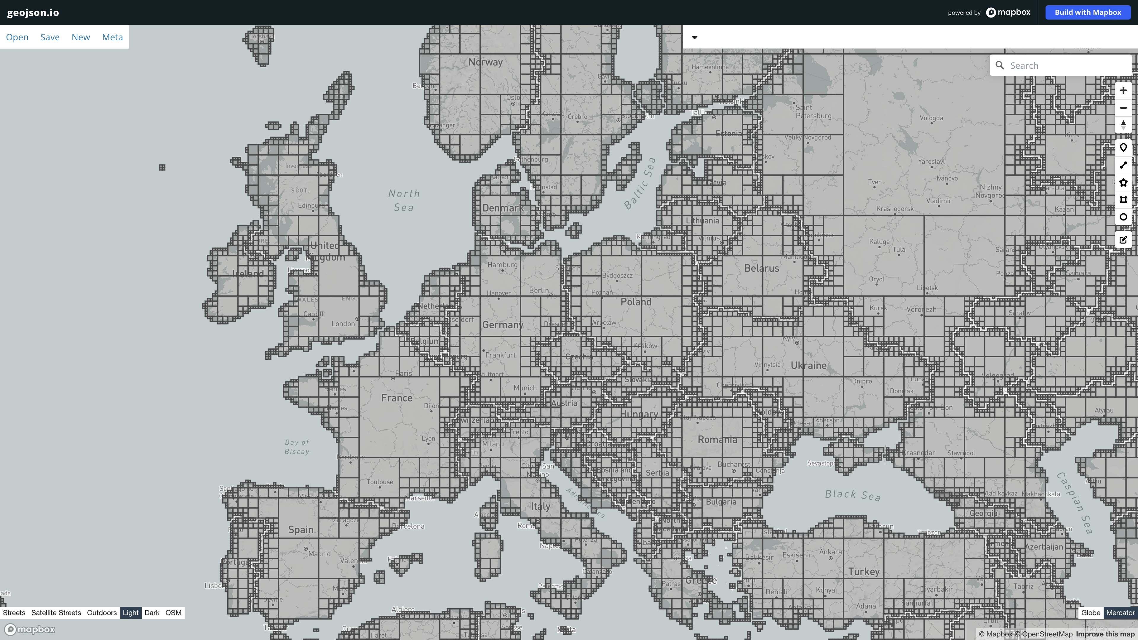
At the beginning, this project was attempted in Go, and the project was open sourced as tzf under the MIT License. The functions for time zone data conversion, data reduction, compression, and indexing mentioned above are all command-line tools, in thetzf/cmd directory. The constructed binary data file is published in thetzf-rel repository, using Go’s embed feature.

After Go is ready, I tried to package into a .so file via CGO for Python to call. Use cibuildwheel to build the wheel of each platform to avoid compiling during installation. There is no problem with the basic test, but it is found that the returned object needs to be recycled manually, otherwise there will be a memory leaktzf#63. However, calling CGO to perform GC from the Python side caused the program to run about twice as slow in some cases. I asked whether there was a more elegant way.

I turned to Rust, good tools such as PyO3 and Maturin, which can be packaged directly into a Python package library without manually recycling objects, and I and I found in some benchmarks that Rust is faster than Go in CPU-intensive scenarios.

So I began to use Rust to load data files, construct map indexes, polygon search and other things in tzf. It is basically smooth. For example, the open sourcegeorust/geo has very rich geo computing functions.

As a result, it took 1,700,000 ns in time zone data processing, compared with 12,000 ns in Go, which is more than 100 times slower. This was likely an efficiency issue in the algorithm implementation, so after an afternoon of wrestling with the compiler, I ported the geo computing function used in Go to Rust. The project is geometry-rs. Rerun the benchmark.

The result took 3,300,000 ns, which was even slower.

What was the reason? First, I tried avoiding object iteration and instead used index values to access elements. At least there is some optimization space in Go. I want to try it, but there is no fluctuation in the result. Then I accidentally noticed that while wrestling with various Rust compiler errors, the point sequence was being passed directly to the function withto_owned, and this object was very large, with millions of points. Replacing this step with a pointer improved performance immediately, to about 30000 ns., because the original Go implementation also constructs an additional layer of pre-indexes within the polygon data, and Rust does not implement this part of the function, so it is acceptable to be slower.

After Rust achieved stable performance, it began to encapsulate the Python library tzfpy with PyO3. The whole process was quite smooth. Lazy initialization is used to initialize the global Finder implementation, so the first call would be slow, and then it would be very fast. That’s it.

Installation and use:

pip install tzfpy

>>> from tzfpy import get_tz
>>> print(get_tz(116.3883, 39.9289))

At present, tzf-rs and tzfpy still use data that is not compressed by Polyline. Later, it will be switched to further compress the binary volume.